Quick Notes on Differentiable Monte Carlo Simulations
Background
If you haven't read my last post and the next paragraph sounds like gibberish, don't worry! None of it is required.
In my last post, I used variance as a proxy for image quality in the loss function. The nice thing about using variance, is that the sum of independent pixel variances is simple to compute (it's just the sum of the individual variances). However, I mentioned one could try using the expected value of a real image quality metric like SSIM instead. Unfortunately computing the expectation of a function like SSIM (or something crazier like NIMA) is not so trivial. One way to compute the expectation of these crazier metrics, would be to use a Monte Carlo techinque. But it was not obvious to me how to get useful gradients out of that procedure.
Problem
Suppose we want to compute a complex expectation. This problem pops in up machine learning in a few places (some ELBO losses for example). Often these problems can be solved using Monte Carlo Sampling.
The basic idea behind using Monte Carlo Sampling to compute expectations is to take:
\(E_{p}[f(x)]\)
and approximate it as follows:
\(E_{p}[f(x)]\) \(\approx\) \(\frac{1}{N} \sum_{i=1}^N f(\overline{\mathbf{x}}_i); \overline{\mathbf{x}}_i\) ~ \(p\)
where the \(x_i\)'s are drawn from the distribution you are sampling over.
If we want to including Monte Carlo estimations inside a differentiable system (such as a neural network) we need a way to differentiate through the simulation.
Easy Mode

Let's start with something simple. If the shape of the probability distribution we are taking the monte carlo estimate over is not a parameter, then differentiating through a Monte Carlo simulation is simple. No adjustments at all have to be made. Mathematically this looks like the following:
\(\frac{d}{d\theta}E_p[f(x, \theta)]\) \(\approx\) \(\frac{d}{d\theta} \frac{1}{N} \sum_{i=1}^N f(\overline{\mathbf{x}}_i, \theta); \overline{\mathbf{x}}_i\) ~ \(p\)
Hard Mode
However often some parameters will affect the shape of the sampling distribution. For example, in my previous post the probabilities of each palette color being chosen per pixel are variables.
Mathemtically this looks like:
\(\frac{d}{d\theta}E_{p(\theta)}[f(x, \theta)]\) \(\approx\) \(\frac{d}{d\theta} \frac{1}{N} \sum_{i=1}^N f(\overline{\mathbf{x}}_i, \theta); \overline{\mathbf{x}}_i\) ~ \(p(\theta)\)
This is where things get a little trickier. I generally found two common ways of approaching this problem.
The Score Function Gradient Estimator (aka REINFORCE)
The idea here is to format the gradient as a second Monte Carlo problem over the same distribution (assuming certain conditions are met). We also make use of the log derivative trick.
\(\frac{d}{d\theta}E_{p(\theta)}[f(x, \theta)]=\frac{d}{d\theta} \int_{\Omega} p(\overline{\mathbf{x}}_i; \theta)f(\overline{\mathbf{x}}_i, \theta)\)
\(\frac{d}{d\theta}E_{p(\theta)}[f(x, \theta)]= \int_{\Omega} \frac{d}{d\theta}p(\overline{\mathbf{x}}_i; \theta)f(\overline{\mathbf{x}}_i, \theta)\) + \(\int_{\Omega} p(\overline{\mathbf{x}}_i; \theta)\frac{d}{d\theta}f(\overline{\mathbf{x}}_i, \theta)\)
\(\frac{d}{d\theta}E_{p(\theta)}[f(x, \theta)]= \int_{\Omega} \frac{\frac{d}{d\theta}p(\overline{\mathbf{x}}_i; \theta)}{p(\overline{\mathbf{x}}_i; \theta)}f(\overline{\mathbf{x}}_i, \theta)p(\overline{\mathbf{x}}_i; \theta)\) + \(\int_{\Omega} p(\overline{\mathbf{x}}_i; \theta)\frac{d}{d\theta}f(\overline{\mathbf{x}}_i, \theta)\)
\(\frac{d}{d\theta}E_{p(\theta)}[f(x, \theta)]= \int_{\Omega} \frac{d}{d\theta}\log(p(\overline{\mathbf{x}}_i; \theta))\)\(f(\overline{\mathbf{x}}_i, \theta)p(\overline{\mathbf{x}}_i; \theta)\) + \(\int_{\Omega} p(\overline{\mathbf{x}}_i; \theta)\frac{d}{d\theta}f(\overline{\mathbf{x}}_i, \theta)\)
\(\frac{d}{d\theta}E_{p(\theta)}[f(x, \theta)]= E_{p(\theta)}[\frac{d}{d\theta}\log(p(\overline{\mathbf{x}}_i; \theta))\)\(f(\overline{\mathbf{x}}_i, \theta)]\) + \(E_{p(\theta)}[\frac{d}{d\theta}f(\overline{\mathbf{x}}_i, \theta)]\)
Pros
- Incredibly simple. Fairly general.
Cons
- Several people seem to agree that high variance is a problem with this method. Tim Vieria calsl the basic method "useless on top of noisy". It seems like controlling the variance is an active area of research.
- You need to be able to represent the derivative of \(p(\overline{\mathbf{x}}_i; \theta)\) analytically (which rules out categorical variables for example).
From what I've seen this approach does not easily fit into an auto differentiation framework
The Reparameterization Trick
As far as I can tell, the reparameterization trick was established by Kingma et al in their paper about Variational Auto Encoders.
The insight here is that some families of distributions can be defined in terms of a differentiable transformation applied to constant underlying distribution. What does that mean?
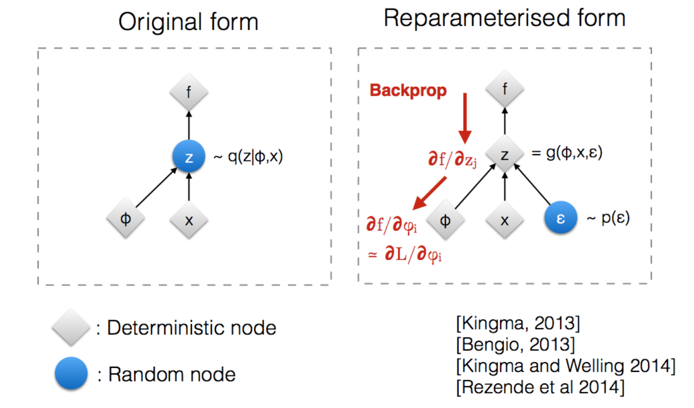
Let's consider the family of normal distributions parameterized by mean \(\mu\) and variance \(\sigma\). Let's say we wanted to differentiate through a function which includes samples drawn from the normal distribution parameterized by the variables \(\mu\) and \(\sigma\). If we approached this directly, we'd have to resort to something like the likelihood trick.
Alternatively, if we draw samples from \(Normal(0,1)\) then multiply the result by \(\sigma\) and add \(\mu\), we can differentiate with respect to \(\sigma\) and \(\mu\) directly through auto differentiation without having to deal with any randomness. This trick works because the normal distribution parameterized by \(\mu\) and \(\sigma\) is equal to the scaled / translated unit normal distribution. Not all distributions have nice properties like this, but for the ones that do reparametrization tricks can be quite nice.
Pros
- Easy to use with existing autodiff frameworks
- At least empirically less variance
Cons
- Not generalizable because you need a specific "trick" per distribution. Not many distributions have one.
The Gumbel Softmax Trick
In my previous post, the random variables I was dealing with were categorical. After learning about the reparameterization trick for normal distributions, I was immediately curious if there was a trick for categorical variables. It turns out there is an approximate one called the Gumbel Softmax Trick.
To understand the Gumbel Softmax Trick we will first talk about the non-differentiable version called the Gumbel Max Trick.
The Gumbel Max trick says that sampling from a categorical distribution with n classes (with probabilities \(p_{1}, ..., p_{n}\)) is equivalent to:
\(argmax_{i \in \{1,..,n\}}\) \(x_i + log(p_i)\)
where the \(x_i\)'s are drawn from a standard Gumbel Distribution. I'm not going to post the derivation of this trick but a walk through can be found here.
The problem with this trick of course is that it's still not differentiable. However we can use a common deep learning trick and replace the discontinuous max with the approximate but continuous softmax function.
\(softmax([(x_0 + log(p_0))/t, ...\)\(, (x_n + log(p_n))/t])\)
\(t\) is an tempreture parameter, which controls how smooth the softmax is. I coded up a quick example of this trick in Jax here if you want to see it in action.
This post is a high level overview but if you're curious, here is some good further reading.
Have questions / comments / corrections?
Get in touch: pstefek.dev@gmail.com