Learn You a NeRF

Posted on 10 January 2023

My NeRF Implementation which generated all the renderings for this post is on github and you can play with it in a minimal colab

A Computer Vision Problem
Over the years computer graphics has gotten really good at rendering virtual worlds. This is known as forward rendering¹. Forward rendering means taking some description of a 3d world stored in a computer and turning it into a realistic looking 2d image captured from a particular perspective inside that world.

The inverse problem, turning an image or collection of images into a 3d scene, is also very interesting. Up until recently these problems were solved in unrelated ways but new techniques called inverse graphics have tied the two problems together. NeRF (Neural Radiance Fields) is a wildly popular² inverse graphics technique which beautifully formulates the problem in terms of forward rendering.

Forward Rendering via Ray Tracing
Before we talk about NeRF, I want to quickly go over the basic ideas of ray tracing, a forward rendering technique. NeRF relies on a very simplified version of ray tracing so understanding the basic ideas behind ray tracing is useful for understanding NeRF. If you already are familiar with ray tracing feel free to skip ahead! For a more comprehensive explanation please see the wonderful Scratchapixel.

The basic idea behind ray tracing is to use a virtual pinhole camera to capture imaginary light rays and turn them into an image. This approximates how cameras work in real life. Below is a diagram of an ideal pinhole camera:

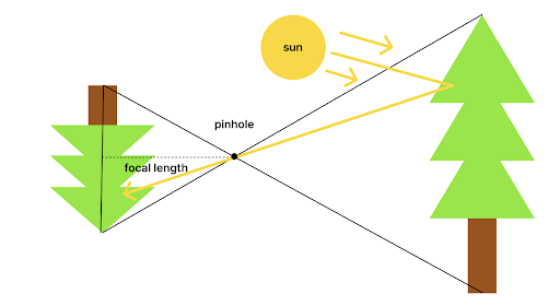
Light from the sun or other light source bounces off of an object and into the pinhole of the camera projecting the object upside down. In our virtual pinhole camera we usually assume the pinhole is infinitely small and has sufficient light exposure so there is no need for a lens and therefore no depth of field effects.

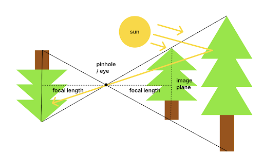
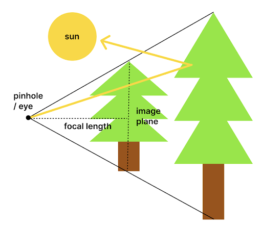
An important notational point is that graphics programmers prefer to talk about rendering in terms of an "eye" placed at the pinhole and an "image plane" placed in front of the camera one focal length³ unit away. This has no real life analog but is the right side up version of the image captured by the pinhole camera so it is easier to work with. Here is a diagram of the image plane:

One way you might try to render an image would be to sample rays of light from the light sources in the scene (the imaginary sun or other lights) and bounce them around until you have accumulated enough inside the pinhole camera to see a finished image. However given the fact that our virtual pinhole is infinitely tiny this would take forever. Even if it wasn't this would be super inefficient as most samples would miss the camera and therefore be useless.

Instead of casting rays from the light source to the camera, we can be more efficient by casting "reverse" rays out from the camera. We can do this because we know that the color of each point⁴ on the image plane is uniquely determined by the light coming into the camera's pinhole from a certain direction. These reverse rays will bounce around the scene until they hit a light source. By the time they have done that they will have followed the exact paths that the incoming light ray from that source would follow and therefore we can determine how much energy is left when that ray of light finally hits our sensor⁵.

One important property of this version of ray tracing I want to highlight is that we can terminate "reverse" rays early and make an approximation of the amount of light coming from the remainder of the tracing process instead of continuing to trace. All ray tracers I'm aware of do this to some extent. Usually there is a max bounce depth before early termination.

The simplest form of this is to terminate immediately when hitting the first object instead of doing any bouncing and make a guess as to the amount of light hitting that object at that particular angle. This is the type of ray tracing NeRF relies on.

So what is NeRF anyway?
Neural Radiance Fields (NeRF) takes in a set of cameras with the following known parameters: position, orientation and field of view as well as the corresponding ground truth photographs taken from each of those cameras. It then learns a 3d representation of the underlying scene. This 3d representation can be used to render the scene from novel viewpoints or turned into a mesh.

NeRF represents the 3d scene with a so-called radiance field. A radiance field can be viewed as two different functions $\mathbf{\sigma(pos)}$ and $\mathbf{c(pos, dir)}$ which together represent a volume.

$\mathbf{\sigma(pos)}$ is a function which takes a position in 3d space and returns the probability density of encountering a particle at that location. This quantity is sometimes called the attenuation but the NeRF authors refer to it as the volume density.

$\mathbf{c(pos, dir)}$ is a function which takes a position in 3d space and a direction then returns the color of light reflecting off that particle. The return type of $\mathbf{c(pos, dir)}$ is a 3 component RGB vector with components from $[0, 1]$.

One thing you might notice is that $\mathbf{\sigma(pos)}$ does not depend on the direction of the ray while the color function does. This is an explicit choice by the NeRF authors, who say that the angle at which you look at an object should not determine whether or not it is there. In contrast the author's acknowledge that the color of the object can be influenced by the ray direction especially if its surface is reflective. For example, consider a mirror, you can look at the same part of it from different angles and you will see different images.

To create a 2d view from this radiance field the authors use a forward rendering technique from an area of computer graphics called volume rendering⁶.

Tracing Rays

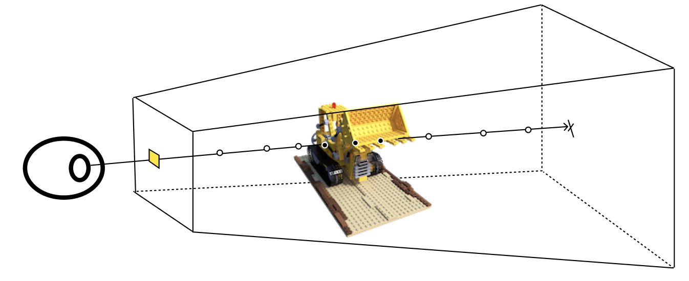
To determine the color of a given pixel in the image plane we take its associated "reverse" ray and trace it through the radiance field.

The main difference between rendering the radiance field and the simple ray tracing we talked about previously is that unlike the simple ray tracing where objects are solid, here we are dealing with objects made of many tiny particles. In this case collisions at any particular point in space are approximated by a probability that they will occur instead of actually computing an intersection test.

Each of the rays we trace passes through the field until it hits a particle (decided by weighted coin flip based on the probability of intersection at each point along the ray) and finally terminates, returning the color reflecting off of that particle towards the camera. Notice there are no light bounces modeled here. As mentioned in the Forward Rendering section the color of the radiance field is serving as an approximation of the light reflected off the particle after the first collision.

Because collisions with the radiance field are probabilistic, casting the same ray over and over again in the same direction will give different colors each time. So instead of casting just one ray per point in the image plane to find its color, we compute the expected color over all possible rays shot from the eye in that particular direction. Since authors don't need to deal with bounces the expected color is fairly simple to compute.

Given the radiance field function, $\mathbf{\sigma(pos)}$ and $\mathbf{c(pos, dir)}$, the expected color for a particular point on the image plane is given by the following equation:

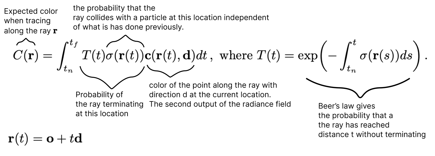
When you understand all the notation this integral is not as scary as it first appears. We are simply computing the expected color of a ray starting from initial position o and direction d going through the radiance field given by $\mathbf{\sigma(pos)}$ and $\mathbf{c(pos, dir)}$.

$\mathit{T(t)}$ is the probability that the ray has not terminated earlier before point $\mathbf{r(t)}$. $\mathit{T(t)}$ is calculated using Beer's law. Scratchapixel has a derivation of Beer's law using differential equations in their volume rendering section.

$t_n$ is the location along the ray of the near plane (the image plane)
$t_f$ is the location of the far plane which is the furthest a ray will go before automatically terminating into the background.

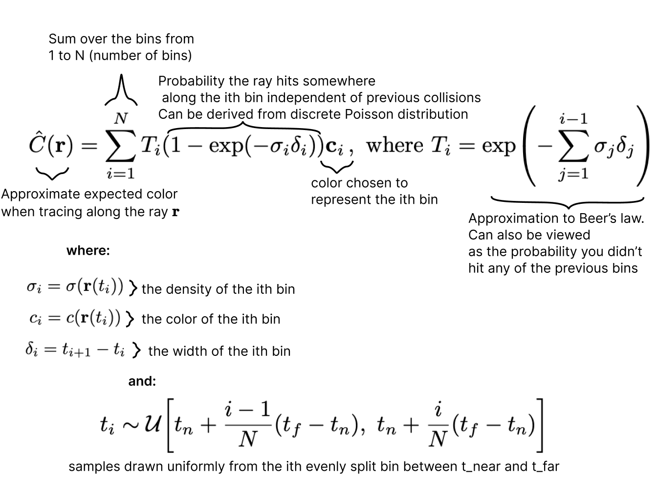
Of course we cannot perfectly calculate the above integral so the NeRF authors choose to approximate it by breaking it up into a sum of a finite number of bins described as follows:

Learning the radiance field
The "neural" part of Neural radiance fields means that the radiance field function will be a neural network. The goal of NeRF is to learn a neural network based radiance field that matches a set of known "training" camera views.

Knowing this let's look again at our radiance field functions $\mathbf{\sigma(pos)}$ and $\mathbf{c(pos, dir)}$. We're going to now refer to them as $\mathbf{\sigma(pos; W)}$ and $\mathbf{c(pos, dir; W)}$. Where $W$ represents the parameters of the underlying neural network approximating the radiance field.

Now let's consider the expected color along a ray $\hat{C}(r)$, from the previous section, which we will now denote $\hat{C}(r; W)$ to explicitly show its dependence on the neural network parameters $W$. Suppose we also know the true color along that particular ray (from a ground truth photograph) denoted by $ground\_truth\_color(r)$.

We can create a loss function between the two values:

$$L(r; W) = (\hat{C}(r; W) - ground\_truth\_color(r))^2$$

Notice that this loss function is differentiable with respect to $W$⁷, the parameters of the neural network. This means that we can use gradient descent to minimize this loss function. If we minimize the sum of the loss over all rays for all known views we can learn a radiance field that faithfully represents the underlying 3d scene. This is the core idea behind NeRF.

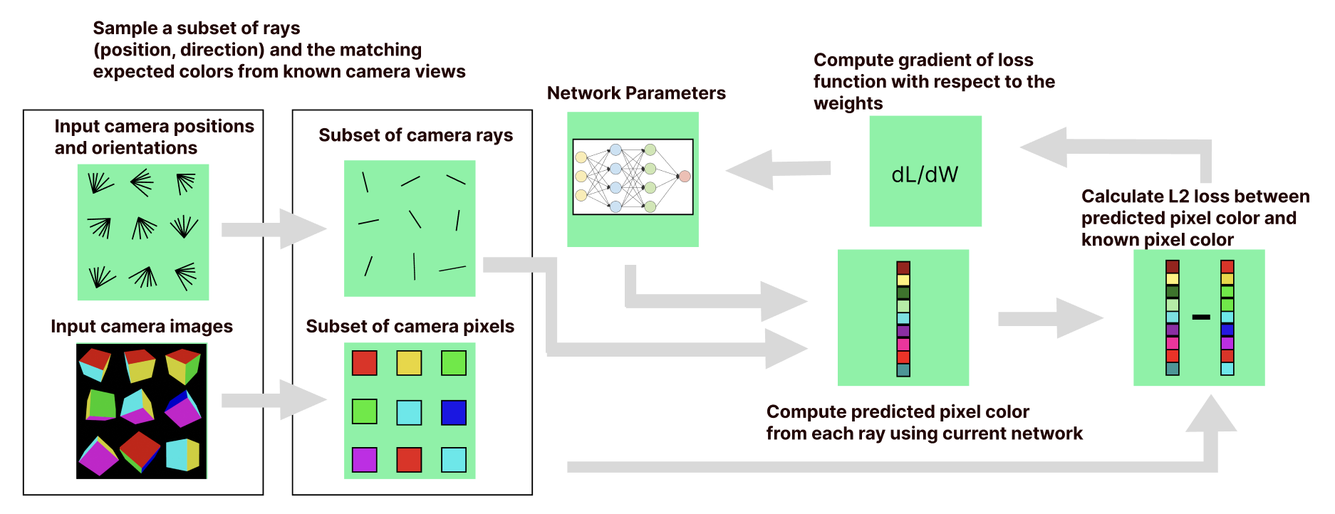
The training process for nerf is pictured above. The basic idea is that for each of our known cameras we can render an image using our current network as the radiance field and then compare the rendered image to the ground truth reference image from the camera. We then take the derivative of the loss with respect to the network parameters⁸ and perform gradient descent to update the network for the next iteration.

In practice rendering an entire image per iteration can be expensive. Instead the authors sample a subset of rays and corresponding pixel colors from each known camera image and roll them all up into a batch. The batch size in the original NeRF paper is 4096 rays. This type of batching is a common technique in deep learning.

It's also important to realize that in the NeRF paper, the neural network learned is tailored to a single scene only.

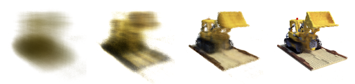
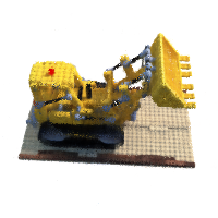
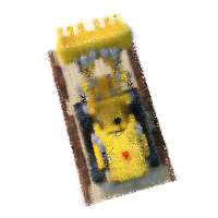
Here are some validation views during the learning process. Note that none of these images are fed into the network at train time, it has never seen the scene from these orientations before:

ground truth

color prediction

depth prediction

Network Architecture
Now let's talk about the actual architecture of the neural network which computes the radiance field.

The network described in the original NeRF paper is a simple feedforward architecture.

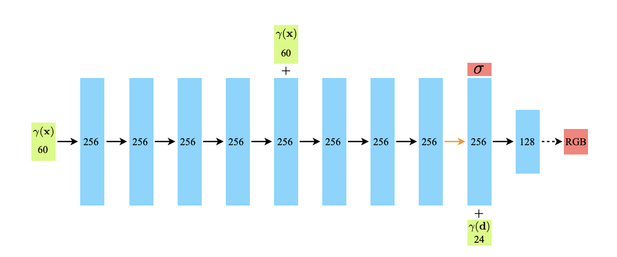
As described in the paper, each black arrow in this diagram represents a connection between layers with a ReLU in between. The dashed arrow is an element wise sigmoid activation and the orange arrow indicates no activation function.

The inputs to the network are the green boxes and the outputs are red boxes.

Initially the position (a vector embedding of size 60) is input at the very beginning of the network and then added in again at layer 5 by concatenating it with the output of layer 4. The idea behind this is that it helps the network "remember" the position in later layers. This is inspired by the skip connections in architectures such as ResNet.

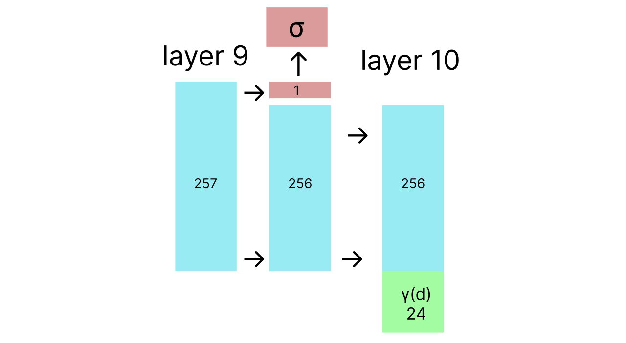
At layer 9 the scalar volume density value $\sigma(pos)$ is output and a ReLU is applied to it to make it non negative⁹. Afterwards the direction embedding (a vector of size 24) is concatenated with the output of layer 9 minus the volume density and input into layer 10 which eventually outputs a 3 element vector representing the r, g and b pieces of the output color at that point looking at that direction.

Very importantly the volume density is output before the direction is added into the network so the volume density remains independent of direction.

High frequency embeddings
When we just talked about the position and direction inputs to the network, I said they had dimensions 60 and 24 respectively. You might be thinking, "That doesn't make any sense. The position and direction are both just 3 dimensional vectors!" So far you would be correct but importantly the authors are not really giving the network just the position and direction vectors. They are giving the network those vectors embedded in a higher dimensional space using a frequency based encoding.

The embedding the authors choose to use for single number p to a point in space of dimension $2L$ is:

The authors apply this embedding function to each of the 3 dimensions of the input vector separately and concatenate the result. They do this for position with $L=10$ and direction with $L=4$.

Importantly when the position is input into this embedding function it has been scaled to be in $[-1, 1]$.

The reason for this embedding is that according to the nerf authors, neural networks are prone to learn low frequency functions. They cite Rahaman et al to back up their claim who also proposes this frequency embedding to remedy the problem. An alternative reason to use frequency embeddings is that the structure of neural networks with only ReLU non-linearities limits the resolution by dividing the scene into polytopes which individually cannot represent non linear details¹⁰.

Hierarchical Sampling
Another problem with NeRF in practice is many of the samples we take will likely hit empty space. If we could more efficiently allocate our samples around actual changes in density we could get better resolution allowing us to capture finer details.

The original paper does this by training two different networks. One "coarse" network and one "fine" network. The coarse network allocates samples using the original bin strategy from our Tracing Rays section. Then the fine network allocates its samples to the same bins based on the relative likelihood of hitting a particle in each bin. The NeRF authors call this inverse transform sampling.

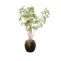
Here's an example of the images rendered using each of the two networks:

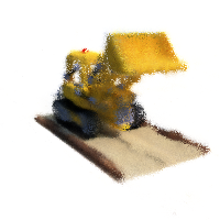
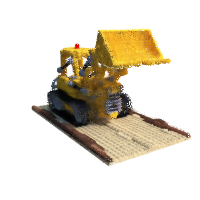
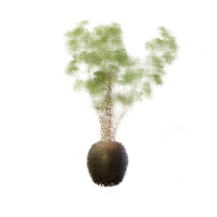
64 coarse network samples
sampled naively

64 fine network samples
from inverse transform sampling

Notice how the coarse network boundaries (left) are fuzzier than the fine network boundaries (right). This is because we are sampling more points around the boundaries from the fine network.

An important implementation detail is the loss from both networks are summed together into the objective function.

Limitations of the original NeRF Paper

Train time
The biggest limitation of the original NeRF paper is the time it takes to render rays. The authors claim an 800x800 image takes 30 seconds to render on a V100 and 1-2 days to train a high resolution radiance field¹¹. Many people have since researched and made enormous progress on this topic. Recently Nvidia's Instant NeRF reduced rendering to 10s of milliseconds and training to mere minutes which is wild given that NeRF is only a few years old.

Rigidity assumption
Another huge assumption the original NeRF paper makes is that the scene it's capturing is static.

One scenario which clearly violates this assumption is reconstructing a moving subject such as a person walking in a video. Works such as Video NeRF try to tackle this problem.

Another slightly more subtle scenario where violations of the rigidity assumption causes problems is when trying to reconstruct static real world objects (such as famous buildings or statues) from crowd sourced pictures. Some violations here include:

The subject of the photo will be different colors during different times of day.
Different cameras have different color ranges and tone mapping
People, cars or other dynamic objects will occlude different part of the object in different photos

Researchers from Google address these problems in NeRF in the Wild. The basic idea is that they learn different networks representing the static details (things that don't change between photos) and transient details in each photo.

By explicitly separating out the static and transient details they can reconstruct objects much more accurately. They also are able to do neat things like arbitrarily change the position of the sun while rendering.

Structural Camera Errors
As we discussed earlier NeRF is based on a pinhole camera model which comes with a host of unrealistic assumptions about the structure of the camera used to take the input photos. It seems like a classic NeRF research project is rebuild NeRF based on a more accurate camera model.

One big assumption is to totally disregard depth of field. It's very possible that depth of field error can be modeled as per camera noise and disregarded by the techniques used in NeRF in the Wild (discussed above) but DoF information could also provide useful clues to estimate the scene. Wu et al build a NeRF which incorporates DoF. They seem to find that it produces sharper radiance fields than vanilla NeRF when used on images with shallow depth of field. However I don't see them comparing their technique to NeRF in the Wild which would be nice. Other papers do similar types of camera corrections such as AR NeRF

Deblur NeRF models a camera with non instantaneous shutter speed to reconstruct radiance fields from motion blurred images more accurately.

MIP NeRF integrates the radiance field over cones instead of rays (equivlant but faster to using multiple samples per pixel) to more accurately capture the underlying field radiance.

Limits of the radiance field
Unlike some differential rendering methods NeRF only predicts depth and color at first bounce in a scene. This means it does not learn deeper structures such as the position of light sources in the scene or unlit object textures. Many followup methods including NeRF in the Wild make strides to learn more of the underlying scene structure.

My Own Journey Implementing NeRF
To further my knowledge of NeRF I didn't just read the paper, I also implemented it in pytorch. As a testament to how good the original paper was, I was able to do it without looking at any of the code. After I finished I was surprised by how structurally different¹² my implementation was from the official repository.

Coding NeRF was an interesting experience. I suspect some of the differences in implementation stemmed from the fact I approach the problem as a programmer trying to break a known algorithm into independent testable pieces rather than a researcher discovering something for the first time (also I am not as good at pytorch so my code is less concise but that's way less fun to say).

Here's a quick summary of what I did:

Created a simple test scene in Blender, a cube with different colored sides¹³
Created basic sampling and ray tracing functions, adding many simple tests.
Made some more complex tests where I rendered a full scene with coarse sampling. For these tests I mocked out the neural network with a hand crafted radiance field representing the same cube I had made in Blender earlier and compared the images my code rendered with the "ground truth" Blender images
Created the neural network and made sure all the tensor dimensions were correct
Tried to learn the cube. This did not work
Did a simple test to see if I could learn a field of all one solid color. That worked
Tried to learn an unlit sphere and found my bug
Rendered the cube successfully on my laptop
Experimented using colab to render on a gpu and realized I hadn't added any gpu support
Added gpu support
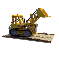
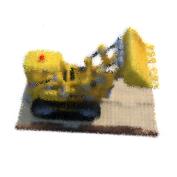
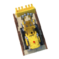
Rendered the lego excavator (resized to 200x200) model on a colab gpu
Implemented the hierarchical network to get better image quality
Rendered the lego model again
Profiled and sped up my implementation¹⁴
Ran a longer run on the lego excavator (again resized to 200x200) on Lambda A100 GPU ($1.10 an hour) for 3 hours

My goal was to build the simplest and most testable parts first, slowly piece them together and finally build and add the neural network itself. The nice thing about rigorously testing each piece was that when I could not learn a sphere in step 7 I knew that the bug had to be in the neural network not in my ray tracing code.

I also got a lot of mileage out of just testing on my laptop before moving to the more complex world of gpus and colab. This allowed me not to worry about the complexities of gpus up front.

Conclusion
I had a great time learning about and implementing the original NeRF paper and will probably try some of the follow up work in the future (especially the real time version). In a world of huge deep inscrutable models with little structure, NeRF is a ray of sunshine. If you've read this far you might also want to consider implementing NeRF yourself! It's not as intimidating as it might seem and it's a great way to practice neural networks and computer graphics.

Thanks to Alex Fox, Laura Lindzey as well as several others for amazing feedback

Have questions / comments / corrections?
Get in touch: pstefek.dev@gmail.com

Corrections
1/18/2022: Fixed the description of Mip-NeRF to say that it does not use multiple samples per pixel

Forward rendering has a different meaning in realtime graphics for video games. This definition has nothing to do with that ↩
Over 50 papers derived from NeRF were submitted to CVPR in 2022. This number is courtesy of Frank Dellart ↩
This is kind of a confusing term in a pinhole camera model since there no lens, hence no "focus". However I can't find a better name for this distance. ↩
I maintain this is technically true for a single point. However in ray tracing we are estimating the color for an entire pixel which is a rectangle, therefore serious ray tracers use techniques such as Monte Carlo sampling to sample many points inside each pixel's rectangle and merge them together to get a final color ↩
If you are scratching your head at how this is accomplished you are absolutely correct. In fact I'd be a little worried if you weren't confused. The answer to this question is incredibly complex and a good chunk of the subfield of computer graphics called Physically Based Rendering is dedicated to creating more and more accurate approximations. A great place to start is the Pbr book ↩
I'm not going to go into detail about volume rendering here (mostly due to my own ignorance). Please look at Scratchapixel's volume rendering section or this chapter of the pbr book for a great introduction ↩
This is a lie for some parts of the function because the neural network in the original paper contains ReLUs but gradient descent still works in practice ↩
No derivative computations are required here because Pytorch's autodifferentiation does it for us! ↩
One problem with rectifying the volume density with ReLU is that sometimes when training the network the ReLU will start "dead" (with a $value \le 0$) at which point the gradient is 0. The network will then make no progress producing all black images. The NeRF authors somewhat solve this problem by adding gaussian noise to the ReLU on their "real world" images but I'm not sure it's addressed fully. ↩
Pure ReLU networks are just the piecewise linear functions over the input space. In the original NeRF paper, the volume density calculated without embeddings is represented by a pure ReLU network. Without any embeddings all the network does to determine the volume density is divide the space into polytopes and do a polytope specific linear prediction based on the x, y and z coordinates to determine the depth. This means non linear details cannot be captured inside a polytope, limiting the resolution. Adding sin and cos makes the network non piecewise linear. ↩
For my renders, I use about 6000 iterations and render at 200x200 resolution which is much faster ↩
Read as "worse" ↩
Fun Fact: I used ChatGPT to help me write this Blender script because I have never used Blender and it was not a focus of this project ↩
Just enough to run at about the same speed as the original paper, speed wasn't a priority for this project. ↩