Optimal Stopping Policies
The Recruiter Problem
Pretend for a minute that you are a recruiter who's looking for people to fill a position. Maybe you're reading this post because I have applied for a position at your company and you're vetting me. Anyways the point is I'm one candidate among many. Even if you interview me and like me how do you know there's not someone better out there to fill the position?
More formally, you are going to interview \(N\) candidates for a job. The order in which they come is random, with all orderings equally likely. After each interview with a candidate you will come up with a quality score (a real number between 0 and 1) for them and then you have to choose whether to hire them on the spot or reject them and hope a better fit comes along. Your goal is to hire the best of the best (the candidate who has the highest score among all N candidates) but you have no idea what the applicant pool looks like (no information about the distribution from which these candidates are drawn). What is the probability that you succeed in your task given that you use the optimal hiring strategy?
This problem is know sometimes as the best choice problem or the secretary problem. We will call it the Recruiter Problem. It is a very famous and well studied problem because of its very surprising solution:
This is a really cool result for several reasons. First of all it's not even clear that there should be any kind of one fits all strategy. Secondly, \(\frac{1}{e} = 0.367879...\) which seems absurdly high. If have a million candidates, you have around a one third chance of choosing the very best one. Here is a graph showing the probability of success using this strategy for different numbers of candidates,
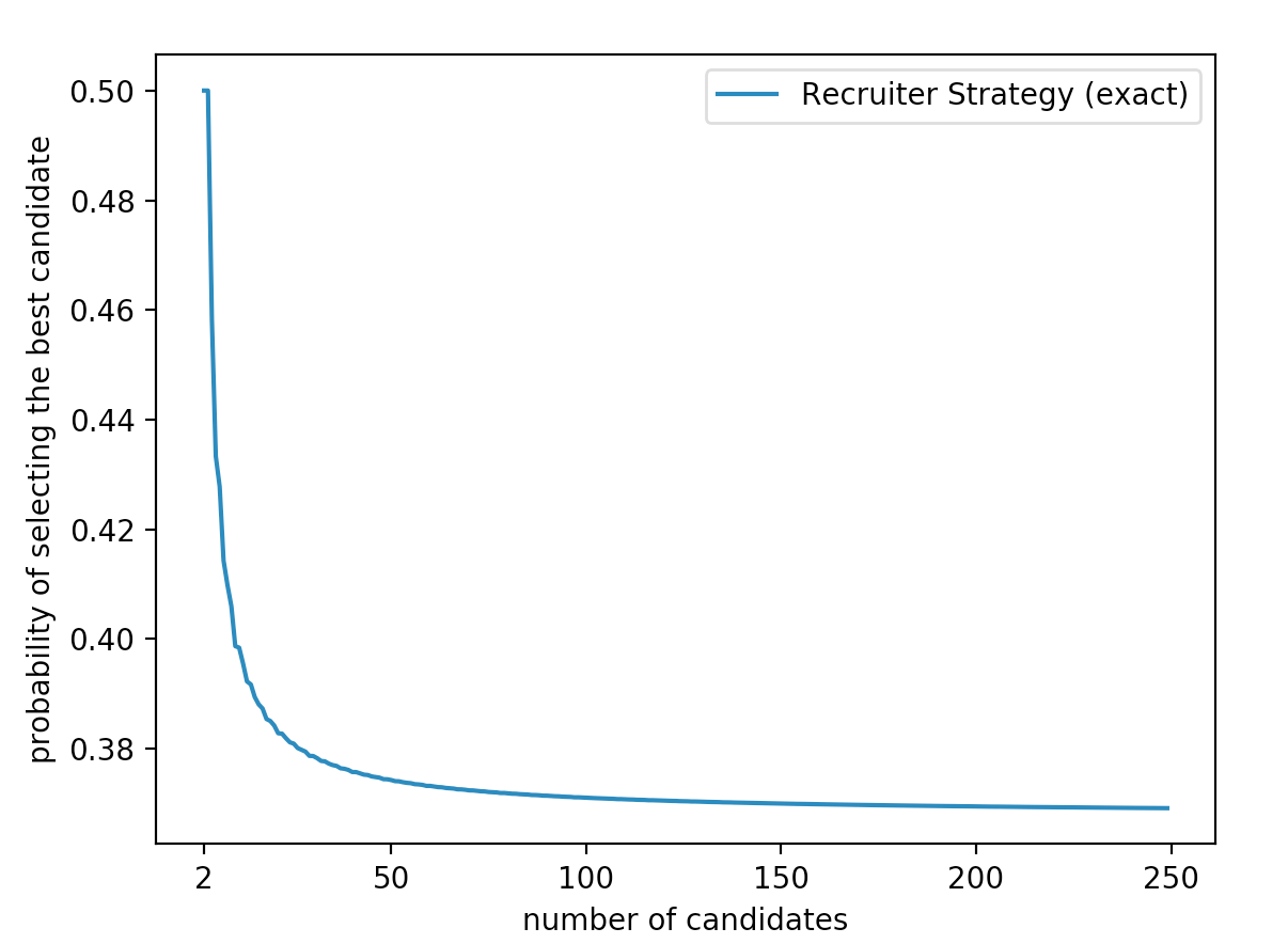
The strategy is also fairly simple and seemingly bizarre.
Strategy
For every N there is an \(r_N^*\) such that the following strategy is optimal. Reject the first \(r_N^* - 1\) percent of the candidates then choose the next candidate who is better all of then them.
This type of strategy is called a cutoff rule. The final surprising fact is that
This means that you see less than half of the many candidates while making your decision.
Analysis
Analyzing the cutoff rule approach to this problem is fairly straightforward. Consider the cutoff rule with a variable \(r\) which defines the cutoff point. The probability of finding the max can be though as follows,
The probability of any applicant being the best if \(\frac{1}{n}\) because our candidates are equally likely to appear in any order. So
The probability of success is clearly zero if when the best candidate is in the first r candidates since we reject them all. So we can simplify the above expression as follows:
Finally we have one last key insight. We can observe that for \(i \geq r\), \(P(\mbox{applicant i is selected} \vert \mbox{applicant i is the best})\) is the same as saying that the best of the first \(i - 1\) candidates is in first r - 1 candidates.
We can observe as \(n \to \infty\) that our probability becomes:
Maxmimizing this function in terms of x gives us \(x^*=\frac{1}{e}\) and \(P(x) = \frac{1}{e}\).
A Savvier Recruiter
It turns out that in the case where we know nothing about the distribution, the cutoff rule is optimal. But what if we do know something? This time let's pretend we know our distribution is uniform on \([0,1]\). We will call this problem the Savvy Recruiter Problem. Now let's try to come up with an optimal strategy for the Savvy Recruiter Problem. After each interview we have to accept or reject the candidate we just interviewed (candidate i). To gain some insight we can take a look at the following statement,
Now we don't have control over the past but we do have the choice between hiring i and rejecting i. Therefore we choose the option which has the highest probability of giving us the best candidate. Let's make a few observations about these probabilities.
If candidate i's score is less than any of the previous candidates we know that:
In this case we would always choose to move on because no matter what our chance of finding the best candidate in the future is we know it is greater than 0.
Now what if candidate i is better than all the other candidates we've seen so far? Off the bat we know that,
This means that,
Let \(q_i\) denote candidate i's quality score. What we want now is the probability that we will not find a better candidate in our last \(N-i\) interviews. Since our candidate scores are drawn from a uniform distribution on \([0,1]\),
So when is it optimal to choose to accept candidate i? It is when,
Equivalently this when,
Using this information we can solve for the threshold \(q^*_i\) such that if \(q_i \geq q^*_i\) our best option is to choose candidate i.
So how much better is a savvy recruiter than a regular recruiter? Below is a graph comparing the probabilities that each type of recruiter will choose the best candidate.
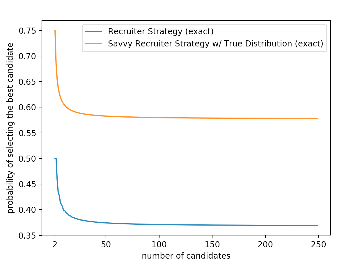
So the savvy recruiter strategy is clearly better for a uniform distribution. This shouldn't be suprising because the savvy recruiter has more information than the basic recruiter. But just to be thorough we want to know if our results would be different if our underlying distribution was not uniform. It turns out it doesn't matter. We can actually transform any distribution into a uniform distribution by looking at percentiles then apply both strategies for a uniform to it. This works in our specific case because we care about finding the best candidate and the transformation into percentiles preserves the order of the candidate values. It's important to note that this type of transformation does not work if we care about maxmimizing other statistics such as expected value. So clearly we have a much better chance of picking the max if we know the underlying distribution from which our candidates are drawn. However in most situations the true distribution isn't usually known (some people would even say that the idea of a single true distribution is ridiculous but we will not address that here for simplicities sake). But what if we could use the information we see during our interviews to appoximate the true distribution? Then we could use the savvy recruiter strategy with the our best guess of the true distribution. Seems kind of cool right? Let's look at an example.
Let's say that you have decided to get a house. However you live in a competitive market so housing tends to go fast. You need a house with in the next month so not a lot of new houses will come onto the market (let's say that you would be able to see a maximum of \(n\) houses). Once you've seen a house, you basically have to decide whether or not to buy it on the spot. By the time you've seen another the first house will probably already be gone. You also want to find the best house for yourself. We will assume we can model the distribution of house qualities around the area with a gaussian distribution but you do not know its parameters (the mean or the variance). So how do you find the best house for yourself?
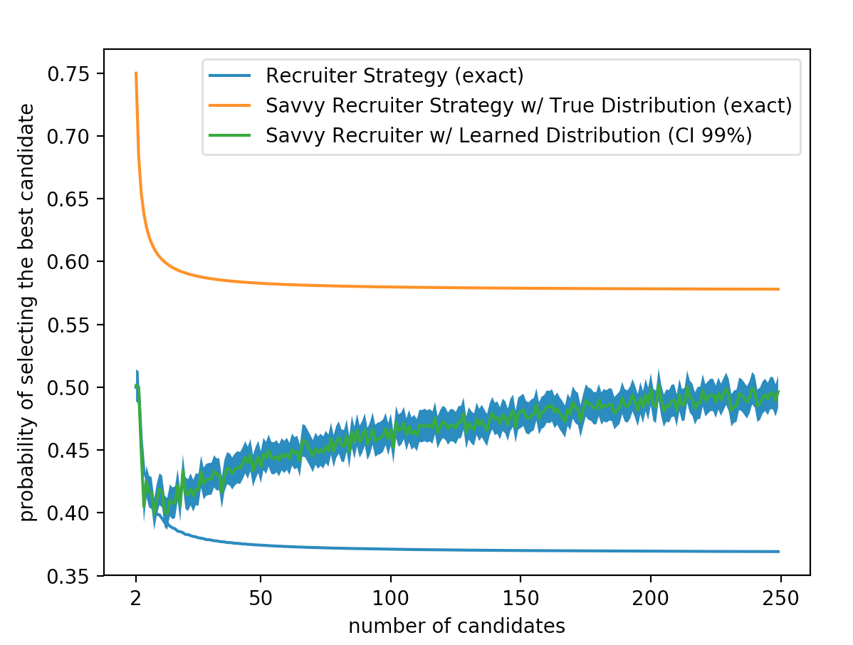
Notice that because each draw is independent the probability of seeing all of them is just the products of the probabilities of seeing each one individually! It turns out that the parameters (\(\mu, \sigma^2\)) which maximize the likelihood of seeing n data points are given by, We can now use these MLE estimates to approach our stopping problem with the optimal strategy for a known distribution. For each candidate house i, we first come up with an estimate of our parameters using all of the houses we have seen so far. Then we use this estimated distribution to calculate the percentile of the candidate house. Finally we check to see if the current candidate is the max we have seen. If so the probability that our candidate house is the best is greater than \(\frac{1}{2}\) we choose it (we can do this the same way as in the thresholding strategy for a known distribution). Here are several graphs demonstrating results of this approach:
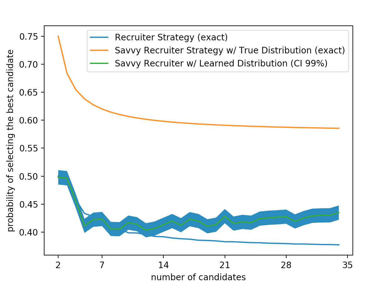
Zooming in we can see that the cutoff policy is on par with the learned policy until there are around 14 houses on the market.
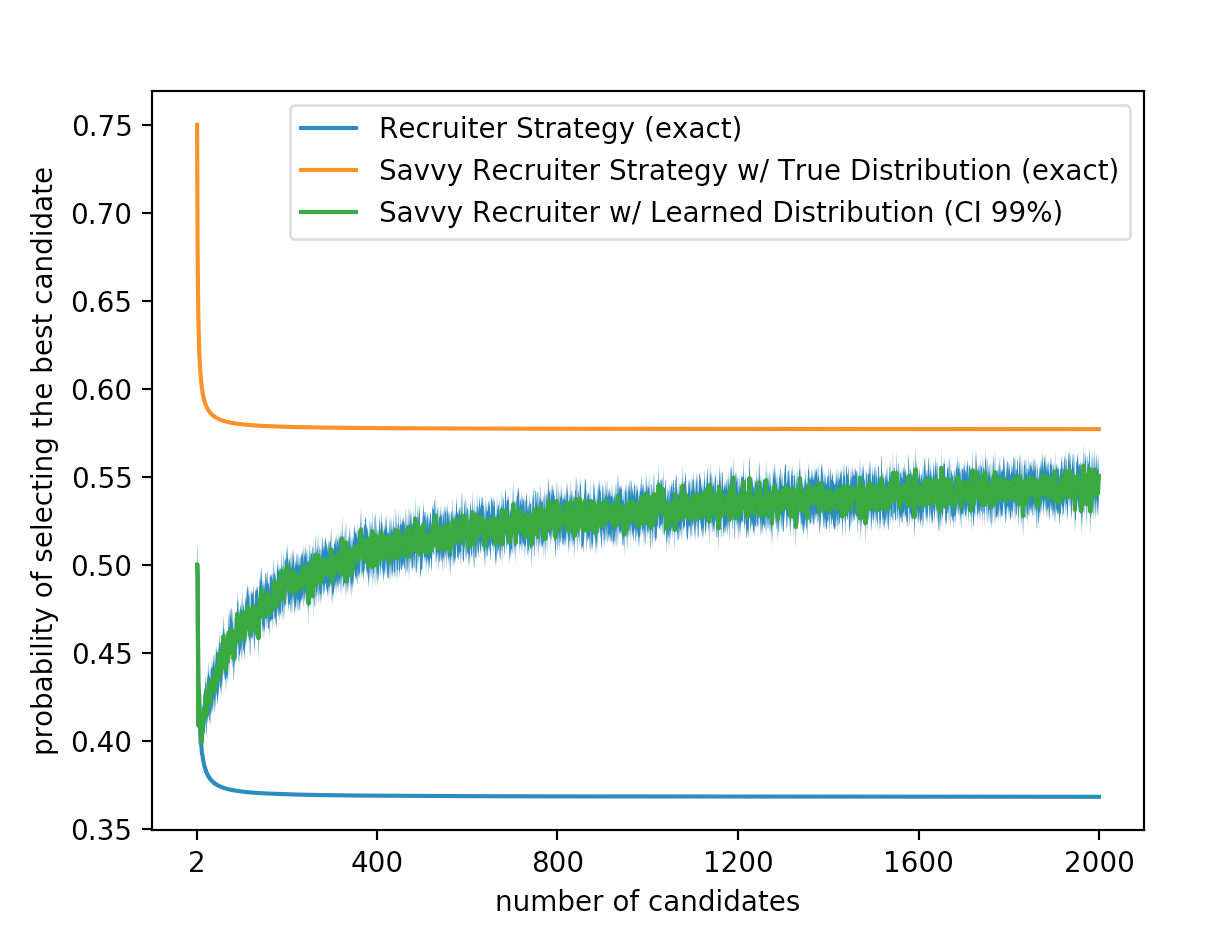
Finally if we look at a much larger number of available houses we can see that the learning strategy gets much better over time.
Limitations(details)
The probability of success of the savvy recruiter strategy is a little more difficult to calculate then that of the basic recruiter strategy. However we will follow the same basic idea. First we break the probability into the sum of the probabilities of succeeding at each step (we can do this because the events are mutually exclusive),
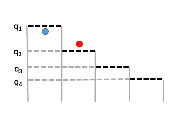
In the above image the current candidate (red) will not be selected even though it is larger than its threshold. To help us out with this problem we will define the true threshold $t_i$. The true threshold $t_i$ is the max of the threshold $q_i$ and the last $i - 1$ candidate values. If the candidate at step $i$ is above the true threshold then they we be picked. So at step i we can condition on the true threshold.
Unchanged Threshold
As we view houses we attempt to learn the true underlying distribution of house qualities. The simplest way to do this is to use a technique called Maximum Likelihood Estimation. Maximum Likelihood Estimation operates on the assumption that each draw from the distribution is independent. It finds the parameters of a distribution (in our case the mean and the variance) which maximize the likelihood of seeing our observed data points.
For a Gaussian distribution the likelihood function is given observed points \(x_1,...x_n\) is defined as follows:(details)
Remember that we are looking for the parameters $\mu, \sigma^2$ which maximize our likelihood function. Now generally products are pretty gross to deal. One common trick when dealing with maximizing products is to maximize the sum of the logs instead. Because log is monotonically increasing function on its domain (and we know the maximum of likelihood function is greater than zero) finding the parameters which maximize the likelihood is equivalent to finding parameters which maximize the log likelihood. For a gaussian distribution our log likelihood function can be derived as follows:
(details)
We run simulations 10000 times (for each n) then average together to get the final probability of success for each n. Each time we run we pick our "true" parameters of underlying normal distribution from two different uniform random distributions. $\mu$ ~ $Unif(0, 1000)$, $\sigma$ ~ $Unif(0, 15)$.
So this is cool little fact but what kinds of problems can we apply it too besides that contrived housing example? Could we use it to made the best stock market trades or decide when to bid on ebay? Unfortunately the answer is no. One large underlying assumption in our model is that the candidate qualities are each drawn independently from an underlying distribution. Many types of time series like the stock market or the price of ebay bids are highly correlated. For example if one tech stock goes down its likely others will have gone down with it. Under these conditions our model would mostly likely work very poorly.