The PCP Theorem and the Hardness of Approximation

Posted on 29 April 2018

Preamble
This post uses a lot of computational complexity terms and is fairly dense. I've included some defintions of frequently used terminology below.

Complexity classes: A complexity class is a set of problems that can all be solved with an upper bounded constraint on a resource based on input size. In this article our constrained resource will usually be algorithmic runtime.
P and NP: P is the complexity class made up of problems that can be solved in polynomial time by a deterministic Turing machine. NP is the class of problems that can be solved in polynomial time by a non-deterministic Turing machine. A major problem in computer science is proving whether or not P=NP. In this post most of the work will be built on the assumption that P $\neq$ NP. If this assumption is false many of our theorems will be irrelevant.
Reductions: A reduction is an algorithm which transforms one problem into another. In this post we will mostly focus on reductions that can be done in polynomial time. A problem is NP-hard if any problem in NP can be reduced to it in polynomial time. Showing that a problem is NP-hard by reducing another NP-hard (or NP Complete) problem to it is a common proof strategy. Notice that showing that a problem is NP-hard does not mean that it is in NP (it could be harder)
NP-Complete: An NP-Complete problem is an NP-hard problem that is also in NP.
Strings and Languages: We can also talk about complexity classes (such as P and NP) in terms of languages which accept certain strings. A language is a collection of strings. For example one language is the language of all strings which contain an odd number of 0s. A more complex example of a language is the set of all strings which represent bipartite graphs (the way we represent graphs as strings is not usually important). Determining whether or not a string is in a given language is now the problem we have to solve. For example we can say that a language $L$ is in P if and only if for any string $x$ we can determine if $x \in L$ in polynomial time.

Probabilistic Checkable Proofs

Probabilistic checkable proofs are a type of complexity class. The basic idea is this, consider a theorem and a lazy student. The lazy student has to decide whether or not the proof is true but does not want to read all of it. In fact the student only wants to read q bits of the proof before going back to sleep. The student also has r quarters (for laundry) next to them on their desk which they can flip (one time per coin) to help make random decisions. Given these r quarters and q bits the student must decide quickly whether or not the proof is true with a high probability.

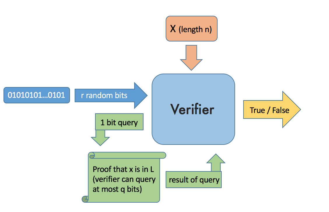
More formally we will first define a probabilistic polynomial time verifier for a language L as follows:
The verifier takes a string x and a proof (that x is in L) as input. The verifier gets to read $q$ bits of the proof and $r$ random bits (drawn from a uniform distribution). Using these two pieces of information the verifier must then decide in polynomial time whether or not x is in L.

Define the complexity class PCP(r, q) as follows:
Let L be a language and v be a probabilistic polynomial time verifier which can read q bits of a proof and has access to string of r random bits drawn from a uniform distribution. Then language L is in $PCP(r,q)$ if and only if
Completeness: For every $x \in L$, there exists a proof that $x \in L$ which v accepts with probability 1
Soundness: For every $x \not\in L$, v accepts all proofs that $x \in L$ with probability at most $\frac{1}{2}$

What does this mean? To gain a basic understanding lets look at some simple edge cases:

$PCP(0,0) = P$ (Claim 1)

Notice $P \subseteq PCP(0,0)$ Let L be any language in P. Since our verifier has polynomial arbitrary steps of computation we can verify that any $x \in P$ with probability 1 without a proof or any randomness by replicating the polynomial time solver for L. Also notice $PCP(0,0) \subseteq P$ because there is no randomness or proof to use. If we could accept any language $L' \not\in P$ then we would have a deterministic polynomial time algorithm which told us if any $x$ was in $L'$. This algorithm creates a contradiction because by definition of $L'$ there is no polynomial time algorithm to determine if any arbitrary string $x$ is in $L'$. $\square$
$PCP(0, O(1)) = P$ (Claim 2)

To show $P \subseteq PCP(0, O(1))$ we can use claim 1 and notice that $P \subseteq PCP(0, 0) \subseteq PCP(0, O(1))$. Now all we have to show is that $PCP(0, O(1)) \subseteq P$. We will use a similar strategy to last time but with a few tweaks. Let's pretend there is a language $L' \not\in P$ but $L' \in PCP(0,O(1))$. In this case we know there is a way to check deterministically in polynomial time whether any $x \in L'$ by only reading a constant number of bits of the proof. Let's call this constant c. One important fact is that c is the same for every $x$. Therefore we can run our polynomial time algorithm on each of the $2^c$ possible bits of the proof in polynomial time (with respect to the size of $x$). If one of these combinations of bits gets accepted then we know $x \in L'$ (completeness) otherwise we know $x \not\in L'$ (soundness). Therefore we have just built a polynomial time algorithm to check if $x$ is in $L'$. This algorithm creates a contradiction because by definition $L'$ there is no polynomial time algorithm to determine if any arbitrary string $x$ is in $L'$. $\square$
$PCP(O(\mbox{log n}), 0) = P$ (Claim 3)

As with the claim 2, we can show $P \subseteq PCP(0, O(1)$ by observing that, $P \subseteq PCP(0,0) \subseteq PCP(O(\mbox{log n}), 0)$. To show $PCP(O(\mbox{log n}),0) \subseteq P$ we will have to again tweak our strategy from before. As before consider an $L' \not\in P$ but $L' \in PCP(O(\mbox{log n},0)$. Unlike last time our verifier's algorithm is not deterministic. However we can make it deterministic by running our verifier's algorithm on every possible random string of r bits. We know that r is $O(\mbox{log n})$ so there are $2^{r}$ combinations which is at most $2^{O(\mbox{log n})} = O(n)$. So we just have to run our polynomial verifier algorithm on a linear number of different random bit strings which gives us a deterministic polynomial time algorithm to check if any $x \in L'$. $\square$

So after looking at all of these cases, what do we think $PCP(O(log n), O(1))$ equals?

PCP Theorem: $PCP(O(log n), O(1)) = NP$

This means that for any decision problem in NP, we can construct a small probabilistic polynomial time verifier which can solve the decision problem up to soundness by at most looking at constant bits of an argument about what the answer is far faster than we could solve the problem deterministically. Seems surprising, right? We will not prove this theorem in this post but we will use it to show some results about how hard it is to approximate certain NP-Complete problems.

MAX-3SAT
3SAT is a famous NP-Complete Problem. It goes like this:
Take a set of m variables and n clauses. Each clause has exactly three literals (variables which may be negated) in it all of them are or'ed together. We then take the conjunction of all of the clauses together. This expression is said to be in 3 conjunctive normal form (3CNF). Here is an example of a 3CNF expression,

$$(x_1 \lor x_2 \lor x_3) \land (\bar x_4 \lor x_1 \lor x_3) \land (\bar x_3 \lor \bar x_2 \lor x_4)$$

The classical 3SAT problem asks if all of the clauses can be simultaneously satisfied.
However sometimes we can't satisfy all of the clauses. MAX-3SAT an optimization problem in which we are given an 3CNF expression and we try to find the maximum number of clauses which can all be satisfied together.

Since MAX-3SAT is NP-Complete we know that we cannot solve it exactly in polynomial time unless P=NP. But what if we could get close?

We say that an problem has a polynomial time approximation scheme (PTAS) if for all $\epsilon > 0$ we can approximate the problem in polynomial time within a factor of $\epsilon$ of the optimal solution. It is important to note however that the runtime of a PTAS must only be polynomial in terms of n (the size of the input) and could be different for different epsilons. For example $O(n^\frac{1}{\epsilon})$ is still polynomial in terms of n. Polynomial time approximation schemes are the only way forward for some NP-Hard problems such as Knapsack and Load Balancing. Sadly, MAX-3SAT has no PTAS.

Theorem: $NP \subseteq PCP(log(n), O(1))$ (PCP Theorem) implies that MAX-3SAT is inapproximable in polynomial time within some $\epsilon > 0$ unless P=NP.

Assume we have a polynomial time approximation scheme for MAX-3SAT. We will show that using this PTAS for MAX-3SAT and a fixed $\epsilon$ we can solve any NP complete decision problem in polynomial time. Let $L$ be the language of strings which satisfy your favorite NP- Complete decision problem. Let $x$ be a string of any size n. We want to know if $x$ is in $L$. Since $L \in PCP(log(n), O(1))$ there is an verifier which takes $x$, log n bits of randomness and a proof that $x \in L$. The verifier reads c (a constant) bits of the proof and then decides whether or not $x$ is in $L$. The completeness property of the verifier says that if $x \in L$ then there is a proof that we can give the verifier so that it will always return true. The soundness property says that if $x \not \in L$ then for every proof the verifier will return true less than half of the time.

For any random string of $O(log(n))$ bits r we can figure out in polynomial time which bits of the proof our verifier will check. Let $Q_r$ be a set of variables corresponding to the locations of each bit our verifier will check. Also define a set of 3CNF clauses $C_r$ with $Q_r$ as its variables. Together the clauses $C_r$ will mimic the output of our verifier (with random string r) when it reads the bits represented by the variables in $Q_r$. It's important that the number of clauses in any $C_r$ does not depend on the size of our input.

(details)

PCP says our verifier only needs to read a c bits of the proof no matter what the size of the input is. In the worst case we could write a CNF formula that maps every possible configuration of the c bits to true or false. In this case we have $2^c$ clauses with c variables per clause. It turns out that we can also translate every CNF instance into a 3CNF instance in polynomial time which means that we may end up with more clauses, but the the number of clauses will still only depend on c not n the size of the input. Therefore this construction is constant in time and space with respect to n.

Now define $Q$ to be the union of all sets $Q_r$ for every possible r and $C$ to be the union of $C_r$. One important fact is that the size of $Q$ and $C$ is linear with respect to n. This is because the size of each $Q_r$ and $C_r$ is a constant and the total number of possible strings r = $2^{O(log(n))} = O(n)$. So the size of $Q,C$ is at most $O(n)$.

Finally create a 3CNF instance whose set of variables is $Q$, and whose set of clauses is the conjunction of all the clauses in $C$. Together all the variables in $Q$ represent a proof $\pi$ (or at least all the parts that our verifier could ever read) that $x \in L$. Each set of clauses $C_r$ represents the output of the verifier with a certain random string r given access to our proof $\pi$. Due to completeness, if $x$ is satisfiable then there is a proof $\pi$ such than all of the clauses will be satisfied.

(details)

Now this is not technically true since we may have broken our larger clauses in small 3CNF clauses. So for example if we broke one clause with 11 terms into 4 different 3CNF clauses then only one of those would have to be satisfied. In cases like this we count all these clauses as one (if one is satisfied then we are happy).

If the proof is incorrect then due to soundness, less than half of the clauses will be satisfied for every proof. If $\epsilon$ is small enough our PTAS have to satisfy more than half of the $C_r$s if and only if our $x$ is in $L$. Notice the same $\epsilon$ works no matter what $x$ is because the size of our construction did not depend on the n. Therefore, a PTAS for MAX-3SAT would give us a polynomial time algorithm to solve any NP Complete decision problem. $\square$

In short what we just did was assume that there was a PTAS for MAX-3SAT. Then we used this PTAS to construct a polynomial time deterministic solver for any NP-Complete decision problem. Because our PTAS takes polynomial time we know that its existence would prove P = NP which in our case is a contradiction (we assume P $\neq$ NP). Part of what makes this proof so cool is that the reduction doesn't change depending on what NP Complete decision problem we use. For maximum confusion I recommend using 3SAT.

The Hardness of Approximating Max Clique
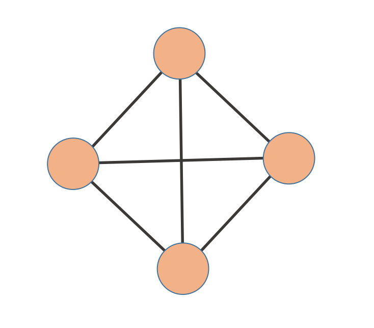
A clique is a set of vertices in a graph which are all connected to each other. The size of a clique is the number of vertices it contains. Here's an example of a clique of size 4

Given a graph G the Max Clique problem is to find the largest clique in G. Max Clique is NP-Complete, which means that it cannot be solved exactly in polynomial time unless P=NP. But can we get close to the optimal solution? In a surprising twist just like MAX-3SAT, Max Clique does not have a PTAS.

Theorem: Max Clique is inapproximable in polynomial time within some $\epsilon > 0$ unless P=NP.

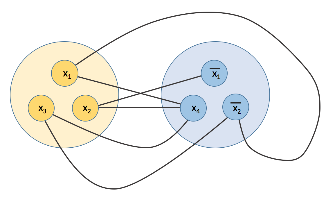
To prove this statement we will show that Max Clique on a certain graph corresponds to MAX-3SAT so closely that if we had a PTAS for Max Clique we would have a PTAS for MAX-3SAT. Heres how we construct this graph. Given a set of $m$ clauses in 3CNF form, we can construct a graph G as follows. For each clause $c_k$ add 3 vertices each one representing a literal in that clause. For every vertex v connect v to every other vertex which is not part of the same clause and that does not represent a negation of the literal v represents. Here is an example of this construction with two clauses,

Let's say we find a clique of size k in this graph. Consider what would happen if we set the variables corresponding to each vertex in our clique to true (or false if they are negations) and all the other variables to false (or true if they are negations). We can do this with no conflicts because by our construction no two vertices in the clique are negations of each other. Also by construction each vertex is in a different clause so at least k different clauses are satisfied.
Now consider $x$ an instance of MAX-3SAT. We know since MAX-3SAT has no PTAS $\exists \delta > 0$ such that we cannot approximate MAX-3SAT within $\delta$. Now choose let our PTAS be an $1+\epsilon$ approximation where $\epsilon < \delta$. We can turn our $x$ into a graph following our construction above. Notice that a $1 - \epsilon$ approximation of max clique gives us a $1 - \epsilon$ approximation for MAX-3SAT. This is a problem because we have just created a PTAS for MAX-3SAT.$\square$

Okay, we can't do construct a PTAS, so we can't get as close as we want. What about approximating MAX Clique within some constant factor? Plenty of NP-Complete problems have a constant factor approximation including MAX-3SAT. As you may have guessed we won't be so lucky with Max Clique.

Theorem: Max Clique has no constant factor approximation unless P = NP.

Before we prove this theorem we have to build up some machinery on graphs. We will do this by defining the strong graph product.

Definition The (strong) graph product on graphs $G = G_1 \bigotimes G_2$ is defined as follows:
$V_G = V_{G_1} \times V_{G_2}$ (where $\times$ is the Cartesian product)
$E_G = \\{(u_1,v_1), (u_2,v_2)\\}$ such that $(u_1, u_2) \in E_{G_1}$ or $u_1 = u_2, (v_1, v_2) \in E_{G_2}$ or $v_1 = v_2$
Here's an example,

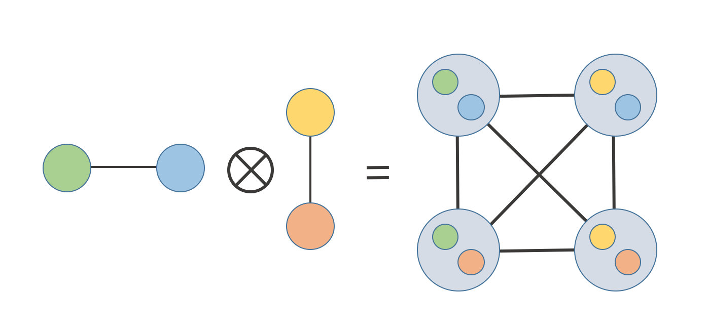
While this definition may seem daunting one can visualize it by imagining that we are putting a copy of $G_1$ at every vertex of $G_2$ then connecting the edges according to our edge rules. Look at the max clique size $\omega(G)$ for each graph in the drawing above:

$$\omega(G_1) = 2, \omega(G_2) = 2, \omega(G_1 \bigotimes G_2) = 4$$

What can we make of this? It turns out that an important fact about graph products is,

$\omega(G_1 \bigotimes G_2) = \omega(G_1)\omega(G_2)$

(details)

Take the two largest cliques $C_1 \in G_1, C_2 \in G_2$. When we take the graph product $G'$ we place a copy of $G_1$ (including $C_1$) at each vertex in $G_2$. Now consider subgraph $G'$ made of the copies of $C_1$ placed at vertices that make up $C_2$. Consider any edge in G' between two vertices $\\{(u_1,v_1), (u_2,v_2)\\}$. Since $C_1$ and $C_2$ are cliques, $(u_1, u_2) \in E_{G_1}$ or $u_1 = u_2$. The same goes for $v_1$ and $v_2$. So our subgraph is entirely connected. The size of this subgraph is $\lvert C_1 \rvert \lvert C_2 \rvert$. Since this subgraph is a clique the max clique has size at least $\lvert C_1 \rvert \lvert C_2 \rvert = \omega(G_1)\omega(G_2)$.

Finally how do we know there is not a larger clique? Well let's reverse our logic. Suppose there is a clique $C' \in G'$ which is larger than $\omega(G_1)\omega(G_2)$. Then we can decompose this clique into one clique in $G_1$ and one in $G_2$. We must be able to do this decomposition because each of if one of the set of vertices that is part of this clique was not a clique itself then we would have a contradiction.

Now we return to showing that Max Clique has no constant approximation. Assume we have an $\alpha$-approximation for Max Clique. Now we know there $\exists \beta > 0$ such that Max Clique cannot be approximated within any factor larger than $\beta$ in polynomial time (Max Clique has not PTAS). Choose a $k$ such that $\beta^k < \alpha$. Take in a graph G. Compute $G^k$ by taking the repeated graph product. Now use our alpha approximation algorithm on $G^k$. Remember our fact from earlier,

$$\omega(G^k) = \omega(G)^k$$

Let $C'$ denote the clique we found. Then we can say:

$$ \lvert C' \rvert = \alpha \omega(G^k) $$

This implies that there is a clique $C$ in our original graph such that:

$$ \lvert C \rvert = \sqrt[k]{(\lvert C' \rvert)} = \sqrt[k]{(\alpha w(G^k))} = \sqrt[k]{(\alpha)}w(G)$$

We know by our definition of k that:

$$ \sqrt[k]{(\alpha)}w(G) > \beta w(G) $$

Therefore we have just created a polynomial approximation for Max Clique within $\epsilon$. Unless P=NP this is a contradiction. $\square$

So it turns out that Max Clique is really bad. In fact the best results on the hardness of Max Clique indicate the the only approximation one can make is a clique of size one (i.e choosing a single vertex).

Getting better hardness guarantees
So far, our results with the standard PCP Theorem have been quite cool. We have used a powerful tool to show that some NP-Complete Problems aren't just hard to solve exactly but are hard to approximate up to a certain point. One question is could we be more specific? It is simple to come up with a $\frac{7}{8}$-approximation algorithm for MAX-3SAT but can we do better? After the PCP Theorem was introduced, researchers have become less interested in proving that there is no PTAS for certain problems and more interested in optimal inapproximability.

Definition An optimal inapproximability result for a problem says there is both an algorithm which is an $\alpha$ approximation that problem as well as a proof that the problem cannot be approximated within a factor of $\alpha + \epsilon$ for any $\epsilon > 0$.

While our classic PCP Theorem was enough to show many problems had no PTAS, it is not quite as simple to use for specific lower bounds. One way to get around this limitation is to define new versions of the PCP Theorem. One such theorem was posed by Johan Hastad:

Theorem (Hastad's 3 Bit PCP): For every $\delta > 0$ and $L \in NP$, there exists a PCP verifier (with $\mbox{log n}$ bits of randomness) such that L can be verified in three queries with completeness $(1 - \delta)$ and soundness at most $\frac{1}{2}+\delta$. Furthermore the tests are of the following form. Our verifier chooses a parity bit $b \in \\{0,1\\}$ and then takes the three bits it queries $q_1,q_2,q_3$ and returns true if:

$$ q_1 + q_2 + q_3 = b \quad (\mbox{mod } 2)$$

A full proof of this theorem is beyond the scope of this post. However we will use this theorem to show optimal inapproxibility results for MAX-3SAT as well as a more specific approximation for Vertex Cover.

MAX-3LIN
The MAX-3LIN problem is defined as follows:
Given a system of integral linear equations (mod 2) with a most 3 variables what is the maximum number of them which can be satisfied simultaneously? It's immediately apparent that this problem is closely related to Hastad's variant of the PCP Theorem.

We can consider Hastad's PCP equivalent to the statement:

For any $\epsilon > 0$ determining between two instance of MAX-E3LIN, one where at least $(1 - \epsilon)$ of the equations are satisfied and one where at most $\frac{1}{2}+\epsilon$ of the equations are satisfied is NP-Hard.

(Details)

If we had a polynomial time algorithm to tell the difference we use it to deterministically test if any string $x$ is in your favorite NP-Complete language L by building a system of equations (one for each possible random string) that mimic our Hastad PCPs output given that string. If we know we satisfied more than $\frac{1}{2}$ of the equations, by soundness we know $x$ must be in $L$, if we don't we know $x$ is not in $L$ by completeness. This argument is very similar to our proof that MAX-3SAT has no PTAS.

Now we will use this formulation to prove better approximation bounds for MAX-3SAT and Vertex Cover. We will call this problem, GAP-3LIN. The GAP part comes from the fact that the domain of all possible numbers of mutually solvable equations has a gap in the middle. In the two proofs we will exploit this gap to give better lower bounds than we would be able to obtain with just vanilla PCP.

Theorem: MAX-3SAT cannot be approximated by a factor of $1 - (\frac{7}{8}+\epsilon)$ for any $\epsilon > 0$.
To show this result we will reduce our gap GAP-E3LIN to MAX-3SAT. Given an equation:

$$ a+b+c = 0 $$

We create the following four clauses:

$$ (\bar a\lor b \lor c) $$

$$ (a\lor \bar b \lor c) $$

$$ (a\lor b \lor \bar c) $$

$$ (\bar a\lor \bar b \lor \bar c) $$

These clauses are important because all four are only satisfied if and only if $a+b+c = 0$ (we can do the same thing if the equation should sum to 1). Otherwise at most $\frac{3}{4}$ of the clauses are satisfiable. From our previous result we know that it is NP-Hard to distinguish between an instance of MAX-E3LIN where $\frac{1}{2}+\delta$ the equations are satisfied versus one where $1-\delta$ of the equations are satisfied for any $\delta > 0$. Consider a polynomial time algorithm Max-3SAT with an approximation ratio of $\alpha$. Take an instance $x$ of MAX-E3LIN and creates a 3CNF expression from it by doing the following. For each equation in $x$ create four clauses following our above model and then combine all of them into one large 3CNF instance. If we could satisfy a fraction of more than $1 - (\frac{1}{2} - \delta)\frac{1}{4}$ of the clauses we could determine between the two different types of GAP-E3LIN instances. Since this is true for all $\delta > 0$, we know that the largest valid value of $\delta$ is 0 (Unless P=NP). This gives us the following lower bound for MAX-3SAT:

$$1 - \frac{1}{8} = \frac{7}{8}$$

$\square$

It turns out that the Hastad PCP Theorem is useful for more than just MAX-3SAT. Another problem which gives a specific constant bound with this theorem is vertex cover.

Vertex Cover Given a graph G we say that a vertex cover of G is a set of the vertices such that every vertex in the graph is directly connected to one of these vertices via and edge, The vertex cover problem is to find a minimum such vertex cover on G.

Independent Set It is useful to talk about independent set whenever we talk about vertex cover. Given a graph G, an Independent Set is a set of vertices which are not connected to each other. The Independent Set problem is to find the largest independent set in G.

Fact One reason why these two problems are often presented together is because one is the complement of the other. That is to say let $I$ the maximum independent set in a graph and let $C$ the minimum vertex cover. $G - I = C$ (or the other way around).

Theorem: Vertex Cover cannot be approximated within a factor of $\frac{7}{6} - \epsilon$ for any $\epsilon > 0$ unless P=NP.

We again use the fact that GAP-3LIN is NP-Hard. Our goal is to use a $\frac{7}{6} - \epsilon$ approximation of Vertex Cover to solve GAP-3LIN. We just need a way to translate equations to graphs. We will do this using the following construction:
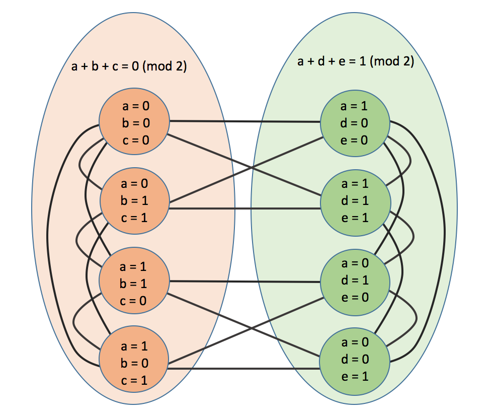
Look at an equation of the form

$$x_1 + x_2 + x_3 = 0 \quad \mbox{mod } 2$$

The first thing we can notice about it is that it has eight possible choices of values. Notice that half of them will satisfy the equation and half of them will not. Therefore for any equation of this form there are 4 ways to satisfy it.
Now in our graph for each equation in our MAX-E3LIN instance we will create four different vertices, one for each of the valid solutions to the equation. We will connect all of them together as well as connecting them to each other vertex in the graph representing a logically incompatible solution to a different equation. When we are done there will be $4m$ vertices. Here's an example with two equations

Observation 1 If at least $(1-\epsilon)m$ of the equations of our GAP-E3LIN instance are satisfiable then our independent set is at least of size $(1-\epsilon)m$. This is because by construction of our graph, each satisfiable equation does not have an edge to any other mutually satisfiable equations because neither of them are different variable choices for the same equation and neither contradict each other. So since the maximum independent set is at least of size $(1 - \epsilon)m$, the minimum vertex cover will be at most of size $(3 + \epsilon)m$.

Observation 2 If at most $(\frac{1}{2} + \epsilon)m$ equations are mutually satisfiable, then our maximal independent set will be of size at most $(\frac{1}{2} + \epsilon)m$. To show this is true consider we will pretend we could have a larger independent set. Take $v$ a vertex in this independent set which does not represent one our our satisfiable equations. By the rules of our construction $v$ would also not conflict with any of the $(\frac{1}{2} + \epsilon)m$ mutually satisfiable equations of the other equations represented in the independent set. Therefore the existence of $v$ would imply there is another equation which could be mutually satisfied. This would contradict our assume that only $(\frac{1}{2} + \epsilon)m$ are mutually satisfiable. So we know that the maximum independent set size is at most $(\frac{1}{2} + \epsilon)m$. This implies that the minimum vertex cover size will be at least $(\frac{7}{2} - \epsilon)m$.

The two observations we have just made help define the gap between vertex cover instances associated with each of the two cases. This means that if we can approximate the upper bound of the smaller case within a factor that is tight enough so our approximation does not overlap with the lower bound of the larger case then we can distinguish between the two cases. To formalize this assume that we have an algorithm which can approximate vertex cover to a factor of $\alpha$. For any $\epsilon > 0$ we know that unless we can solve GAP-3LIN in polynomial time:

$$\alpha (3 + \epsilon) > \frac{7}{2} - \epsilon$$

$$\alpha > \frac{\frac{7}{2} - \epsilon}{(3 + \epsilon)}$$

This is to say that if $\alpha$ is too small than our smaller case and our larger case still be distinguished in our approximation. Because this is true for all $\epsilon > 0$ we can take the limit as $\epsilon \to 0$ to find an $\alpha$ that works for all cases:

$$\alpha = \frac{\frac{7}{2}}{3} = \frac{7}{6}$$

$\square$

Let's Play a Game
Now we have seen some basic ideas such as gaps and simple graph operations as ways to prove hardness. One more common set of tools to show hardness of approximations is 2 Prover 1 Round Games. This last section aims to give some background on this problem.

Definition: A 2 Prover 1 Round Game is a game played by two provers (players) with the following parameters:
Two sets of questions: (one for each player) $X,Y$
A probability distribution: $\lambda$ over $X \times Y$
A set of answers: $A$
A verifier (acceptance predicate): $V:X\times Y \times A \times A$
A strategy for each player: $f_1:X \to A, f_2:Y \to A$

The rules of the game are as follows:
The verifier picks two questions $(x, y) \in X \times Y$ from the distribution and asks x to player 1 and y to the player 2.
Each player thinks of an answer to their respective questions $(a_1,a_2)$ by computing $a_1 = f_1(x), a_2 = f_2(y)$.
The verifier takes both answers and the original questions $v(x,y,a_1,a_2)$ and returns either true or false.

The goal of both players is to maximize $\omega(G)$ to be the optimal win probability for the game G.

Also it is important that the two players cannot communicate during the game.

You might be thinking, what kind of stupid game is this? Why don't computer scientists at least play something cool like fortnite? Well here's something kind of cool. We can formulate many problems as 2 Prover 1 Round Games. Let's give an example using good old 3SAT.

Given a set of clauses $x$ in 3CNF form, consider the following 2P1R game:
Let $X$ be the set of all clauses in $x$.
Let $Y$ be the set of all variables in $x$.
Let $\lambda$ be such the variable we draw from $Y$ will be in the clause drawn from $X$ (it will be one of the three of them with uniform probability).
Our first prover will return an assignment $\alpha$ of variables satisfying the clause $c_j$ it was given. The second prover will return an assignment $\beta$ of $x_i$ the variable it was given. The verifier will return true if and only if $\beta$ matches the assignment given to the same variable in $\alpha$.

Observation 1: If $x$ is fully satisfiable then both players just pick according to the satisfying assignment. In some cases there may be more than one satisfying assignment in which case both players can agree some sort of ordering scheme beforehand and pick the first one.

Observation 2: If no satisfying assignment exists then every assignment fails to satisfy a certain factor of the clauses (let's call it $p$). Then the probability of failure will be at least $\frac{p}{3}$.

Now there are several things that are interesting about this 2 prover round 1 game reduction. One is that we turned 3SAT which is a decision problem into a gap decision problem. The second thing which is related is that we can now start to talk about this game in terms of completeness and soundness. In a way this is starting to sound like the PCP Theorem.

Another thing we could try is to play some kind of repeated game. One way we could do this is asking a series of questions, one after another. However it turns out to be more interesting to ask a bunch of questions at the same time (in parallel). We define a parallel n-repeated game $G^n$ for some 2P1R game G to be similar to G but each player reads a tuple of n questions and then outputs a tuple of n answers. The verifier accepts if and only if all the individual answers would be accepted by the verifier for G. So what can we say about these repeated games?

Theorem (Parallel Repetition Theorem): For all games $G$ if $\omega(G) = 1 - \delta$ then,

$$ \omega(G^n) \leq 2^{-\Omega(\delta^3 n)} $$

While we will not go talk about this theorem much it is interesting because it can be used to decrease the size of gaps. In our 3-SAT game it is NP-Hard to distinguish between cases where we succeed with probability 1 and probability $1-\frac{p}{3}$. But what if we could make our gap smaller? This could potentially make it easier to show different approximations are hard.

Summary
In this post I have summarized my findings after researching the a few basic concepts surrounding the PCP Theorem. Throughout this post there are a few big ideas. First we looked at the PCP Theorem itself and the ideas of completeness and soundness. We played with a few toy cases to get a feel for what the statement was saying. Next we used the PCP Theorem to shows MAX-3SAT had no PTAS. In this proof we turned our random PCP verifier in to a deterministic instance of MAX-3SAT. Then we showed that using MAX-3SAT we could search for a proof that our statement was correct or not. We then used graphs and the self improvement property of the graph product to prove that Max Clique had no constant approximation. After that we looked at Hastad's 3 bit PCP and used it to get a few more specific bounds on MAX-3SAT and Vertex Cover. The most important part of these proofs were the gap preserving reduction from our GAP-MAX-E3LIN decision problem. Finally we looked at a totally different way of viewing everything as a game. These general proof strategies give us some tools to tackle inapproximability arguments.

Exercises to the Reader

1) Show $PCP(log(n), 1) = P$

Hint

Think about our proof that MAX-3SAT has no PTAS.

Answer

As a proof of this consider our reduction in the proof for MAX-3SAT having no PTAS. We constructed a MAX-3SAT instance which checked if there was a (the bits of the proof were the variables) proof which could satisfy every one of the O(n) possible combinations of our O(log(n)) bits of randomness. The key was that we only had to have a constant number of variables because we only read a constant number of bits of the proof. Furthermore the size of our clauses was based on the number of bits we read. If we do this same construction here we will end up with an instance of MAX-1SAT which is solvable in polynomial time.

2) We talked about MAX-E3LIN but never proved any hardness results for it. Use Hastad's PCP Theorem prove the following:
Theorem: MAX-3LIN cannot be approximated by a factor of $\frac{1}{2}+\epsilon$ for any $\epsilon > 0$.

Answer

Reduce the optimization version of MAX-E3LIN to the decision version using a gap preserving reduction.

3) When the repeated version 2 Prover 1 Round Game was originally conceived it was conjectured that

$$\omega(G^k) = \omega(G)^k$$

Give a 2P1R Game which shows that this is false (i.e. $\omega(G^k) > \omega(G)^k$)

Answer

We define the Feige Game defined as follows:
Each player gets a bit as input. They must output a bit and a player. The players win if their bits are the same and that player did get that bit. Because they can't communicate $\omega(G) = \frac{1}{2}$. The best strategy is to agree upon a player in advance. That player will pick themselves and their bit and the other player will guess their bit. However if the players play the two round version they can double down on their original bets which would mean $\omega(G^2) = \frac{1}{2}$ as well.

Sources (and great references for learning more):
http://www.cs.jhu.edu/~scheideler/courses/600.471_S05/lecture_9.pdf
http://people.seas.harvard.edu/~madhusudan/courses/Spring2016/scribe/lect18.pdf
http://pages.cs.wisc.edu/~shuchi/courses/880-S07/scribe-notes/lecture29.pdf
http://www.cs.princeton.edu/~zdvir/apx11slides/guruswami-slides.pdf
https://cstheory.stackexchange.com/questions/18360/multi-prover-verifier-games-and-pcp-theorem
http://theory.cs.princeton.edu/complexity/ab_hastadchap.pdf