Optimizing an Open Source Texture Synthesis Library
Background
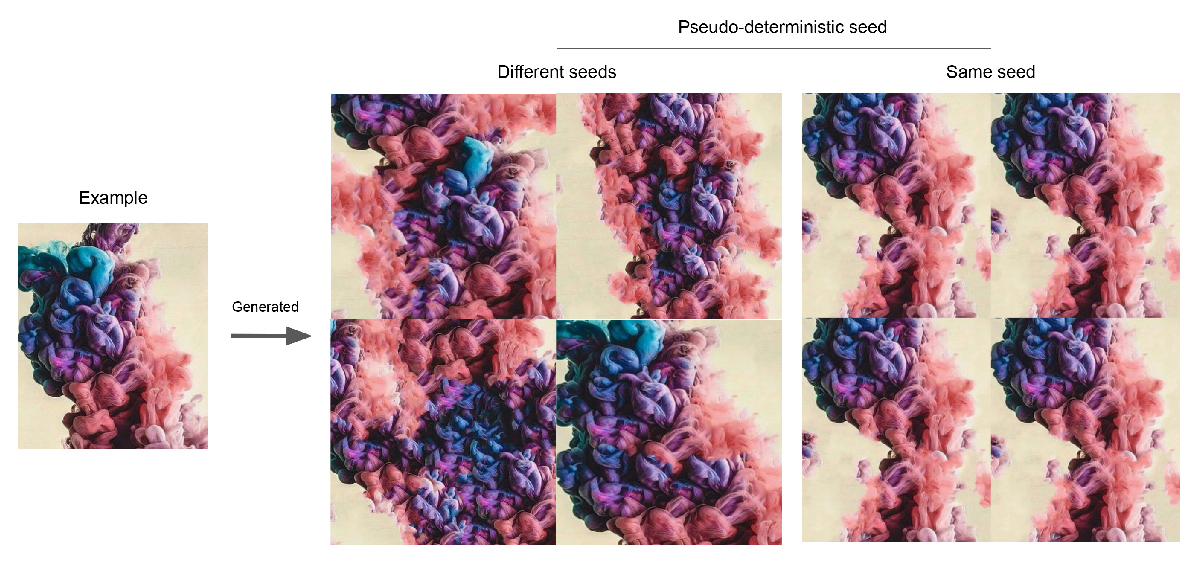
Near the end of 2019 I stumbled across this talk by procedural generation researcher Anastasia Opara. In the talk she presents a novel algorithm for example based texture synthesis. The goal of example based texture synthesis is to take one or more example textures and synthesize a new visually similar output texture.
Here's an example from the project README:
I was really curious about this algorithm and wanted to see if I could make it run faster as an exercise in profiling.
Embarking on a Journey
While I'm not going to go into great detail about how the algorithm works (see Anastasia's talk if you're curious!) it's helpful to understand the basic idea.
We start with an empty output image and seed it with a few random pixels from our example images.
Then repeat the following procedure until the output image is filled:
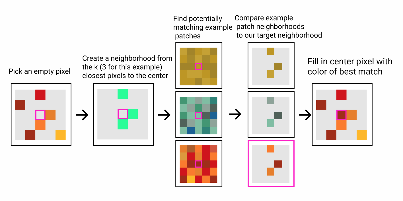
1. Choose an empty pixel in the output image. We will call this the center pixel.
2. Find the k closest non empty pixels to the center in the output image. Note in the first few steps there might be fewer than k pixels in the entire output image. The locations of these k pixels relative to the center pixel define a neighborhood.
3. Come up with a list of the most promising neighborhoods in the example image(s)
4. Compare the most promising candidate neighborhoods in the example image(s) to the neighborhood around the center pixel and pick the most similar one.
5. Fill the center pixel in the output image with the color of the center pixel in the best matching neighborhood.
One last important detail is that the algorithm works on filling multiple empty pixels in parallel to take full advantage of multi core cpus.
Missteps and Micro optimizations
Now it was time to optimize. The first thing I did was to run the program on a few sample inputs with the xcode instruments profiler (partly because it was new to me). I even found a cool library which made it easier to use instruments with rust. Using instruments I was able to see how much each instruction contributed to the overall runtime of the program.
Being able to see time per instruction was perfect for me because I was looking for micro optimizations. I'm using the term micro optimization here to mean a very small change which has a relatively large impact compared to its size. Even though they are not always a good idea, micro optimizations seemed like the best place to start because they would be less of an investment on my end. I also didn't know if the project maintainers would be excited about large code changes.
Looking at the profiler output I was drawn to this line which looked like an unnecessary array resize operation nested within our once per pixel loop.
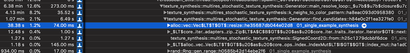
An important note about interpreting the numbers above is that this algorithm runs in several passes and is divided among multiple threads. The image above only shows one pass which accounts for about 12.6% of the runtime of the entire program. However each pass contains the highlighted instruction and behaves similarly. To get a rough estimate of the true impact of this instruction these percentages should be multiplied by a factor of about 8 (100/12.6). So the highlighted instruction really accounts for about 9.5% of the total program runtime.
After I eliminated the unnecessary array resize instruction I ran the program through the profiler again which seemed to confirm that it had gotten about 10% faster which I figured was pretty good for a first try. Of course, the profiler adds some overhead to the program, so to truly confirm that my optimization worked I needed to run it on a couple of examples without any profiling. When I did this I was shocked to see no improvement.
So what was happening? It turns out the cargo-instruments command I was running compiled the program in debug mode by default which turned off significant optimizations. When I built the program in release mode the unnecessary array resize was automatically removed. I learned two very important lessons from this: First, of all when you benchmark you have to think carefully about what exactly you're benchmarking. Secondly, the compiler is smart and makes some micro optimizations for you.
A little embarrassed and somewhat defeated, I went back to the drawing board.
I grabbed a couple more profiles making sure this time to use release mode. After poking around some more I found that a significant amount of time was being spent loading pixels from the source images into intermediate buffers which were later used for neighborhood comparisons step of the algorithm.
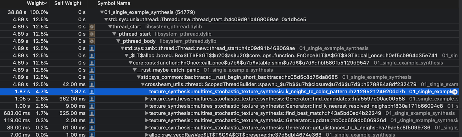
Again using the same runtime adjustment from the last profiling section this function seemed to take about 37.6% of the total runtime. I suspected cache misses were a significant contributor here, but regardless of the actual problem source I knew that reading the neighborhood pixels for each candidate was expensive.
Of course the algorithm still needed to do the candidate neighborhood comparisons so I couldn't completely eliminate reading each candidate's neighborhood pixels. Luckily for me there was already a related optimization in the project,
This related optimization targeted the actual comparison step when finding a best candidate neighborhood. In the comparison step each candidate neighborhood was assigned a score by summing up the differences (always positive) between it's pixels and the target's neighborhood pixels. It turned out that often you could stop summing up these differences early if you already knew this current candidate's score was going to be higher than the best candidate's score so far.
Once I understood this I just extended the idea to avoid reading the pixels needed for the unnecessary comparisons by removing the intermediate buffers and reading pixels only as they were needed which seemed to greatly reduce the average number of reads. I tested my optimization on a few different laptops with several output sizes using references images from the repository as inputs. It seemed like I had improved performance by around 15-25% depending on the output texture size, reference images and the computer I was using.
Quantifying performance impact was a lot harder than I thought it would be. There were so many different parameters to the program that could affect performance: size of the reference image(s), size of the output images, number of threads. Hardware differences were also a huge factor. If I were really being rigorous I would have tried to put together a large collection of images and output sizes to benchmark off of. Due to time and budget constraints I did not assemble a super rigorous benchmark but my appreciation for the problem of performance testing has grown tremendously.
Once I was confident that my micro optimization worked I made my first pull request. It was accepted but to my surprise the performance gains that the reviewers saw were not nearly as good as the ones I did. When one of them benchmarked it on an AMD Threadripper (with 64 virtual cores) the speed up was so small it might have just been noise.
Blocking And Locking
At this point I decided to use some Google Cloud free trial credits I had lying around to spin up some larger machines to test on. Using a 64 core machine I noticed that just like on the thread ripper I didn't see much of a performance improvement from my micro optimization. I tried multiple tests with different numbers of threads (from 0 up to 64) and saw that as the number of threads increased the performance gain from my optimization dropped.
So in my mind there were two explanations. First was that my optimization didn't save as much time when there were multiple threads. Second was that there was another source of latency which increased with the number of threads and that simply got so big it drowned out any noticeable effects of my optimization. It turned out this second explanation was correct.
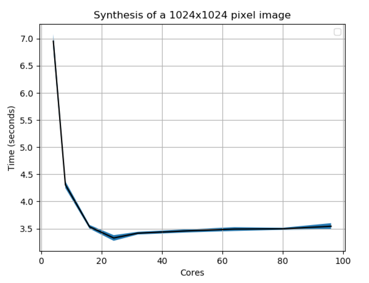
The additional source of latency turned out to be thread contention. To get the k nearest neighbors for each candidate pixel the algorithm was using a data structure called an r*tree. An r*tree provides a way to efficiently store points for nearest neighbor lookups. Exactly how an r*tree works is not actually super important here. The problem was that there was only one r*tree shared across the entire image. To prevent race conditions the r*tree had been wrapped in a read-write lock. This type of lock allows parallel reads but writes must happen in series. Reads also cannot occur while a write is in progress. With large numbers of threads, writing became a large bottleneck. Looking at a graph of program runtime versus number of cores also helps illustrate this effect.
What I realized is that after a few pixels had been filled in the chance that one of the k nearest neighbors would be super far away from the candidate pixel was negligible. So I broke the images in to a grid of r*trees. The basic idea was that writes in two close cells could still block but writes in two far away cells could now be done in parallel. More details can be dound in my second pull request. To see the improvement from this change we can look at this graph below of synthesis speeds before / after:
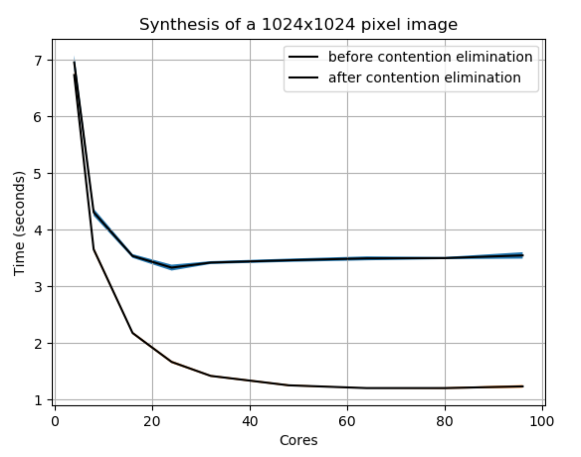
An important note here is that the improved version does not scale linearly either. In an ideal world maybe it would but there are several complicating factors that are at play here. First of all the program has some initialization costs as well as having to synthesize the first few pixels in series. Both of these steps cannot be parallelized. Secondly contention is complicated and can crop up in many places. I believe I did eliminate a large source of contention but I'm sure there is more that could be done. Finally this algorithm is not embarrassingly parallel and will ultimately have to have some amount of informtion shared between threads.
Tricks and Trade Offs
Overall I was pretty excited by how this project turned out. However I think it's worth noting that there are often some tradeoffs which are made during optimizations. A common one that I saw in this project was trading speed for flexibility. Austin Jones, a previous contributor, had also made some significant speedups. One of them was to replace some function evaluations with a lookup table. This resulted in a large speed up but it came at the cost of limiting the range of input values to 8 bits per pixel because larger ranges of numbers would cause the size of the lookup table to explode. My tree grid optimization was somewhat similar in the fact the structure was two dimensional. Although I think it could be extended to three dimensions, it would have to change at least a little if Embark wanted the library to generate voxel models or something. So the lesson here is to wait until your functionality is set in stone before you try to heavily optimize it.
Acknowledgements
While I said many things above about optimization and profiling I am no expert and always looking to learn more so if you think something is incorrect or have any suggestions feel free to get in touch!
Also a big thanks to the people at Embark Studios who were nice enough to take the time to review my code / ideas!
Have questions / comments / corrections?
Get in touch: pstefek.dev@gmail.com